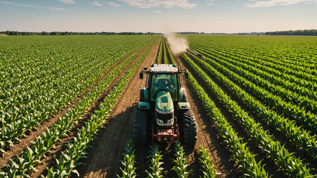
The gap between "the satellite shows stress in zone 4" and "I have a prescription file loaded in the applicator controller" is where most precision ag programs stall. The data is there. The equipment can execute variable-rate applications. But the translation step, from spectral anomaly to agronomic prescription to controller-compatible file, is where operations with no dedicated agronomy staff get stuck.
This is a workflow problem as much as a technology problem, and it has a tractable solution.
Step 1: Confirm the stress type
A variable-rate application map needs to be built around a specific input and a specific agronomic rationale. NDVI depression in zone 4 doesn't tell you whether to apply nitrogen, sulfur, fungicide, or nothing. The prescription starts with the stress type identification, which requires either ground truthing (tissue sample, field observation) or high-confidence AI hypothesis with historical context.
The Croploom analysis output provides the hypothesis (nitrogen deficiency, water stress, disease pressure, equipment damage) along with the confidence level. A high-confidence nitrogen hypothesis in a wet-spring year with known soil drainage issues in that zone is sufficient to proceed to prescription without a field visit. A low-confidence or multi-hypothesis output typically warrants a tissue sample first.
Step 2: Define the treatment zone boundaries
For a variable-rate prescription to execute correctly, the zone boundaries need to match the spatial resolution capabilities of your application equipment. Most John Deere and Case IH variable-rate controllers can respond to zone boundaries at 3 to 5 meter resolution at field operating speeds. Finer boundaries don't get executed accurately.
The Croploom prescription export generates zone boundaries at the resolution that matches your equipment class, not the satellite's raw pixel resolution. A Sentinel-2 pixel is 10 meters. A Planet pixel is 3 to 5 meters. The zone boundaries in the prescription are generalized to your equipment's actuator response distance, which prevents prescription zones that your controller physically can't execute.
Step 3: Set the prescription rates
This is the agronomic judgment step that no satellite system can fully automate. The prescription rate for a nitrogen side-dress application in zone 4 depends on the current crop growth stage, the prior application rate, the soil organic matter in that zone, the season's rainfall pattern, and the expected yield potential. Those inputs come from your agronomist or your farm management records, not from satellite imagery alone.
What Croploom provides is the zone-specific rate adjustment: zone 4 needs 15 to 25% more nitrogen than the field average based on the stress severity and zone size, scaled to your base rate. Your agronomist or your own historical records establish the base rate. The satellite data refines the spatial allocation.
Step 4: Export and execute
The prescription file exports to ISO-XML (the standard precision ag prescription format) compatible with John Deere Operations Center, Climate FieldView, and most third-party precision ag platforms. If your controller reads prescription files directly via USB in a different format, the Croploom support team can generate the conversion on request.
The whole workflow from anomaly detection to prescription file takes about 20 to 40 minutes with a confirmed stress hypothesis. That's the practical time budget you should expect for in-season variable-rate prescriptions built from satellite data, not days and not instant.
Closing the loop: tracking prescription response
The step that most variable-rate programs skip is tracking whether the prescription actually worked. Without a feedback loop, you can't know whether the zone-specific rates you applied produced the intended yield response, or whether the boundaries were correct, or whether the input rate was calibrated appropriately for that zone's typical response.
The Croploom yield-response tracking overlays the prescription file with post-harvest yield monitor data from the same field season. For each treatment zone, it calculates the yield relative to the field average and the yield relative to the same zone in prior seasons. That comparison tells you whether the variable-rate application moved the needle in the direction you expected, and by roughly how much.
Over three to five seasons of tracking, that data builds a zone-specific calibration history. A nitrogen-deficient zone in the northwest corner that received a 20% rate uplift in the first year and showed a 12-bushel yield response has a different optimal rate in year two than it would if you were making the prescription from scratch. The historical response data narrows the rate uncertainty and improves the economic return on every subsequent application in that zone.
When to use in-season versus pre-season prescriptions
Not all variable-rate prescriptions need to be built in-season from satellite data. Pre-plant nitrogen prescriptions, seeding rate maps, and lime applications are most efficiently built from stable zone data -- historical NDVI stacks, soil ECa surveys, or yield monitor history -- during the winter months when there's time for the agronomic analysis to be thorough.
In-season satellite prescriptions add the most value for decisions that are genuinely in-season: side-dress nitrogen timing and rate, foliar micronutrient applications responding to an observed deficiency, fungicide application decisions tied to observed disease pressure, or any situation where the agronomic decision depends on what's actually happening in the field right now rather than on pre-plant assumptions. The key is matching the prescription workflow to the decision type, and not forcing every precision ag application through the same data pipeline regardless of whether it warrants in-season or pre-season inputs.